Word of the Day

Topology

DEFINITION:

The field of mathematics concerned with spatial properties that are preserved under continuous deformations of objects (such as stretching, bending and morphing, but not tearing or gluing).

HISTORY:

Read it here…

https://www.britannica.com/science/topology

If you want to learn more watch this…

REFERENCES:

https://www.storyofmathematics.com/glossary.html

https://www.britannica.com/science/topology

Simultaneous equations

DEFINITION:

A set or system of equations containing multiple variables which has a solution that simultaneously satisfies all of the equations (e.g. the set of simultaneous linear equations 2x + y = 8 andx + y = 6, has a solution x = 2 and y = 4).

HISTORY:

Read it here…

https://www.britannica.com/science/simultaneous-linear-equation

If you want to learn more watch this…

REFERENCES:

https://www.storyofmathematics.com/glossary.html

https://www.britannica.com/science/simultaneous-linear-equation

Riemannian geometry

DEFINITION:

A non-Euclidean geometry that studies curved surfaces and differentiable manifolds in higher dimensional spaces

HISTORY:

Riemann developed a type of non-Euclidean geometry, different to the hyperbolic geometry of Bolyai and Lobachevsky, which has come to be known as elliptic geometry. As with hyperbolic geometry, there is no such thing as parallel lines, and the angles of a triangle do not sum to 180° (in this case, however, they sum to more than 180º). He went on to develop Riemannian geometry, which unified and vastly generalized the three types of geometry, as well as the concept of a manifold or mathematical space, which generalized the ideas of curves and surfaces.

If you want to learn more watch this…

REFERENCES:

https://www.storyofmathematics.com/glossary.html

https://www.storyofmathematics.com/19th_riemann.html

Zermelo-Fraenkel set theory

DEFINITION:

The standard form of set theory and the most common foundation of modern mathematics, based on a list of nine axioms (usually modified by a tenth, the axiom of choice) about what kinds of sets exist, commonly abbreviated together as ZFC.

HISTORY:

ZFC is the basic axiom system for modern (2000) set theory, regarded both as a field of mathematical research and as a foundation for ongoing mathematics (cf. also Axiomatic set theory). Set theory emerged from the researches of G. Cantor into the transfinite numbers and his continuum hypothesis and of R. Dedekind in his incisive analysis of natural numbers (see [a5] or [a10]). E. Zermelo [a20] in 1908, under the influence of D. Hilbert at Göttingen, provided the first full-fledged axiomatization of set theory, from which ZFC in large part derives. Although several axiom systems were later proposed, ZFC became generally adopted by the 1960{}s because of its schematic simplicity and open-endedness in codifying the minimally necessary set existence principles needed and is now (as of 2000) regarded as the basic framework onto which further axioms can be adjoined and investigated. A modern presentation of ZFC follows.

If you want to learn more watch this…

REFERENCES:

https://www.storyofmathematics.com/glossary.html

https://www.encyclopediaofmath.org/index.php/ZFC

Type theory

DEFINITION:

An alternative to naive set theory in which all mathematical entities are assigned to a type within a hierarchy of types, so that objects of a given type are built exclusively from objects of preceding types lower in the hierarchy, thus preventing loops and paradoxes.

HISTORY:

In a letter to Gottlob Frege (1902) Russell announced his discovery of the paradox in Frege’s Begriffsschrift. Frege promptly responded, acknowledging the problem and proposing a solution in a technical discussion of “levels”. To quote Frege:

Incidentally, it seems to me that the expression “a predicate is predicated of itself” is not exact. A predicate is as a rule a first-level function, and this function requires an object as argument and cannot have itself as argument (subject). Therefore I would prefer to say “a concept is predicated of its own extension”.

He goes about showing how this might work but seems to pull back from it. As a consequence of what has become known as Russell’s paradoxboth Frege and Russell had to quickly amend works that they had at the printers. In an Appendix B that Russell tacked onto his The Principles of Mathematics (1903) one finds his “tentative” theory of types. The matter plagued Russell for about five years.[3]

Willard Quine presents a historical synopsis of the origin of the theory of types and the “ramified” theory of types: after considering abandoning the theory of types (1905), Russell proposed in turn three theories:

the zigzag theory
theory of limitation of size,
the no-class theory (1905–1906) and then,
readopting the theory of types (1908ff)

Quine observes that Russell’s introduction of the notion of “apparent variable” had the following result:

the distinction between ‘all’ and ‘any’: ‘all’ is expressed by the bound (‘apparent’) variable of universal quantification, which ranges over a type, and ‘any’ is expressed by the free (‘real’) variable which refers schematically to any unspecified thing irrespective of type.

Quine dismisses this notion of “bound variable” as “pointless apart from a certain aspect of the theory of types”.

The 1908 “ramified” theory of types

If you want to learn more watch this…

REFERENCES:

https://www.storyofmathematics.com/glossary.html

https://www.revolvy.com/page/History-of-type-theory

Zeta function

DEFINITION:

A function based on an infinite series of reciprocals of exponents (Riemann’s zeta function is the extension of Euler’s simple zeta function into the domain of complex numbers).

HISTORY:

In 1859 Riemann published a paper giving an explicit formula for the number of primes up to any preassigned limit—a decided improvement over the approximate value given by the prime number theorem. However, Riemann’s formula depended on knowing the values at which a generalized version of the zeta function equals zero. (The Riemann zeta function is defined for allcomplex numbers—numbers of the form x + iy, where i = Square root of√−1—except for the line x = 1.) Riemann knew that the function equals zero for all negative even integers −2, −4, −6, … (so-called trivial zeros), and that it has an infinite number of zeros in the critical strip of complex numbers between the lines x = 0 and x = 1, and he also knew that all nontrivial zeros are symmetric with respect to the critical line x = ¹/₂. Riemann conjectured that all of the nontrivial zeros are on the critical line, a conjecture that subsequently became known as the Riemann hypothesis.

EXAMPLES:

If you want to learn more watch this…

REFERENCES:

https://www.storyofmathematics.com/glossary.html

https://www.britannica.com/science/Riemann-zeta-function

Diophantine equation

DEFINITION:

A polynomial equation with integer coefficients that also allows the variables and solutions to be integers only.

HISTORY:

Because little is known on the life of Diophantus, historians have approximated his birth to be at about 200 AD in Alexandria, Egypt and his death at 284 AD in Alexandria as well. Diophantus married at the age of 33 and had a son who later died at 42, only 4 years before Diophantus’ death at 84. He is best known for his work, Arithmetica , which contains 13 books “consisting of 130 problems giving numerical solutions to determinate equations (those with a unique solution) and indeterminate equations” (Diophantus). The method he formulated for solving later became known as Diophantine analysis. From his book, Arithmetica , only 6 of the 13 books have survived. Scholars who studied his works concluded that “Diophantus was always satisfied with a rational number and did not require a whole number” (Diophantus). He did not deal with negative solutions and only required one solution to a quadratic equation, which was what most of the Arithmetica problems led to (Diophantus). Brahmagupta was the first to give the general solution of the linear Diophantine equation ax + by = c (Boyer 221). Diophantus did not use sophisticated algebraic notation. He did, however, introduce an algebraic symbolism that used an abbreviation for the unknown he was solving for (Diophantus). He also gained fame from another book called On Polygonal Numbers . Diophantus’ methods of solving problems have had both lasting effects and great benefits for the studies of algebra and number theory.

EXAMPLE:

Solve the equation

First we examine gcd(97,35). We have

This means that gcd(97,35)=1. Now we go backwards and express gcd(97,35) as a linear combination of 97 and 35:

that is

If we multiply this equation by 13 we get

which means that one solution of the diophantine equation is x=169, y=-468. This is however not the only solution. We can exactly as in part 3 add and subtract the least common multiple

such that

We thus have infinitely many solutions

If you want to learn more watch this…

REFERENCES:

https://www.storyofmathematics.com/glossary.html

http://www.ms.uky.edu/~carl/ma330/projects/diophanfin.html

http://staff.www.ltu.se/~larserik/applmath/chap10en/part4.html

Gaussian curvature

DEFINITION:

An intrinsic measure of the curvature of a point on a surface, dependent only on how distances are measured on the surface and not on the way it is embedded in space.

HISTORY:

The Hanover survey work also fuelled Gauss’ interest in differential geometry (a field of mathematics dealing with curves and surfaces) and what has come to be known as Gaussian curvature (an intrinsic measure of curvature, dependent only on how distances are measured on the surface, not on the way it is embedded in space). All in all, despite the rather pedestrian nature of his employment, the responsibilities of caring for his sick mother and the constant arguments with his wife Minna (who desperately wanted to move to Berlin), this was a very fruitful period of his academic life, and he published over 70 papers between 1820 and 1830.

EXAMPLE:

If you want to learn more watch this…

REFERENCES:

https://www.storyofmathematics.com/19th_gauss.html

https://www.storyofmathematics.com/glossary.html

Euclidean geometry

DEFINITION:

“Normal” geometry based on a flat plane, in which there are parallel lines and the angles of a triangle sum to 180°.

HISTORY:

During the fourth and third centuries B.C.E., an Alexandrian Greek named Euclid wrote The Elements, in which he laid down the foundations for working with various two-dimensional and three-dimensional shapes in a study now called geometry. Although most of what he wrote had been discovered before by other mathematicians. Euclid was important because he was the first person to systematize all of the previous observations on geometry into a single coherent system. It was called Euclidean geometry in his honor, though today it is also known as plane geometry, or the study of shapes on flat surfaces.

Euclid realized that a rigorous development of geometry must start with the foundations. Hence, he began the Elements with some undefined terms, such as “a point is that which has no part” and “aline is a length without breadth.” Proceeding from these terms, he defined further ideas such as angles, circles, triangles, and various other polygons and figures. For example, an angle was defined as the inclination of two straight lines, and a circle was a plane figure consisting of all points that have a fixed distance (radius) from a given centre.

As a basis for further logical deductions, Euclid proposed five common notions, such as “things equal to the same thing are equal,” and five unprovable but intuitive principles known variously as postulates or axioms. Stated in modern terms, the axioms are as follows:

1. Given two points, there is a straight line that joins them.
2. A straight line segment can be prolonged indefinitely.
3. A circle can be constructed when a point for its centre and a distance for its radius are given.
4. All right angles are equal.
5. If a straight line falling on two straight lines makes the interior angles on the same side less than two right angles, the two straight lines, if produced indefinitely, will meet on that side on which the angles are less than the two right angles.

EXAMPLE:

In the given figure, $∠ a a n d ∠ b$ are:

-Alternate interior angles-

For more examples watch this…

If you want to learn more watch this…

REFERENCES:

https://study.com/academy/lesson/euclidean-geometry-definition-history-examples.html

https://www.britannica.com/science/Euclidean-geometry

https://www.storyofmathematics.com/glossary.html

Magic square

DEFINITION:

A square array of numbers where each row, column and diagonal added up to the same total, known as the magic sum or constant (a semi-magic square is a square numbers where just the rows and columns, but not both diagonals, sum to a constant).

HISTORY:

The earliest known magic square is Chinese, recorded around 2800 B.C. Fuh-Hi described the “Loh-Shu”, or “scroll of the river Loh”. It is a typical 3×3 magic square except that the numbers were represented by patterns not numerals.

Although this may be the first record, it seems likely that others played with numbers to make the “first” magic square. Probably, many early humans discovered them independently. They may have played with piles of stones on a pattern in the sand or they may have stacked nuts on leaves layed out as a square grid. It seems somewhat improbable that it required a single mathematical genius in 2800 B.C. to develop the first simple 3×3 magic square.

Since then, certainly, many people in many nations have enjoyed, studied, and recorded magic squares. For further details of early records see See Mark Farrar’s Website, and David Singmaster’s Chronology of Recreational Mathematics

EXAMPLE:

magic sq 1 — 3 x 3 Magic Square with 15 as Magic Constant

For more examples watch this…

If you want to learn more watch this…

REFERENCES:

https://www.grogono.com/magic/history.php

https://study.com/academy/lesson/what-is-a-magic-square-in-math-history-examples.html

Least squares method

DEFINITION:

A method of regression analysis used in probability theory and statistics to fit a curve-of-best-fit to observed data by minimizing the sum of the squares of the differences between the observed values and the values provided by the model.

HISTORY:

Gauss was the first to define the method of least squares was contested in his day. Adrien-Marie Legendre first published a version of the method in 1805. In short, Gauss pushed his definition to the extreme in a way that Legendre hadn’t. And, it was Gauss who won the great comet debate.

On January 1, 1801, an Italian astronomer named Giuseppe Piazzi discovered the comet Ceres and was able to maintain visual tracking of its position for forty days at which time it disappeared behind the sun. The problem of the day then became determining when the comet would reappear from behind the sun’s glare without having to go through the complicated renderings of planetary motion. Figuring out the comet’s position became an intense competition with many of the renowned minds of the time vying for best guess.

EXAMPLE:

Fit a least square line for the following data. Also find the trend values and show that ∑(Y−Yˆ)=0.

X	1	2	3	4	5
Y	2	5	3	8	7

Solution:

X	Y	XY	X2	Yˆ=1.1+1.3X	Y−Yˆ
1	2	2	1	2.4	-0.4
2	5	10	4	3.7	+1.3
3	3	9	9	5.0	-2
4	8	32	16	6.3	1.7
5	7	35	25	7.6	-0.6
∑X=15	∑Y=25	∑XY=88	∑X2=55	Trend Values	∑(Y−Yˆ)=0

The equation of least square line Y=a+bX

Normal equation for ‘a’ ∑Y=na+b∑X 25=5a+15b —- (1)

Normal equation for ‘b’ ∑XY=a∑X+b∑X2 88=15a+55b —-(2)

Eliminate a from equation (1) and (2), multiply equation (2) by 3 and subtract from equation (2). Thus we get the values of a and b.

Here a=1.1 and b=1.3, the equation of least square line becomes Y=1.1+1.3X.

For more examples watch this…

If you want to learn more watch this…

REFERENCES:

https://www.storyofmathematics.com/glossary.html

https://blog.bookstellyouwhy.com/carl-friedrich-gauss-and-the-method-of-least-squares

https://www.emathzone.com/tutorials/basic-statistics/example-method-of-least-squares.html

Julia set

DEFINITION:

The set of points for a function of the form z² + c (where c is a complex parameter), such that a small perturbation can cause drastic changes in the sequence of iterated function values and iterations will either approach zero, approach infinity or get trapped in loop.

HISTORY:

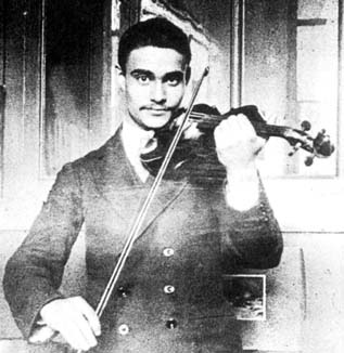
Julia Sets: Gaston Julia playing the violin

Julia sets are named after Gaston Julia. (He is depicted in the photo as a young man—one of the few photos available before he suffered a disfiguring facial wound in World War I). He was a French mathematician who discovered Julia sets and first explored their properties. He lived from 1893 to 1978 and his masterpiece on these sets was published in 1918 (Julia).

His interest apparently was piqued by the 1879 paper by Sir Arthur Cayley called “The Newton-Fourier Imaginary Problem” (Peitgen et al. 1992 p. 775). Cayley was studying the equation f(z) = z³ + c = 0, using the Newton-Fourier iterative method to seek the roots. Since there are three roots, he wondered if one could predict which of the three roots a given starting value of z would reach as a limit. He could not answer this question and commented that the problem “appears to present considerable difficulty” (Peitgen et al. 1992 p. 774). The solution, made apparent with modern computer iterative techniques, is that there are “basins of attraction” for each of the roots, such that a starting value of z falling in, for example, basin 1 will reach root 1 as the limit. But the shape of these basins is infinitely complex:

Julia Sets: Basins of attraction — Basins of attraction

Here the three basins of attraction are colored green, yellow, and blue respectively, and are seen to be intricately interconnected. In fact, further magnification of this image, e.g., using the program WinFract.exe (see Works Cited), demonstrates that the complexly interwoven pattern continues for all magnifications. Note that the diagram illustrates a somewhat more complex Julia set with underlying expression f(z) = z – ((z³ – 1)/3z²).

Julia did not live long enough to see a satisfactory visualization of the myriad and complex forms his sets take on—complexity in fact exceeding that exhibited by the Cayley problem. The creation of images of Julia sets and of other complex dynamical systems requires computer technology not readily available to him, and early attempts to depict them were very crude (Peitgen et al. 1992 p. 123).

EXAMPLE: